Codebooks and Workflow
Download .Rmd (won’t work in Safari or IE)
See GitHub Repository
What Are Data?
Data are the core of everything that we do in statistical analysis. Data come in many forms, and I don’t just mean .csv, .xls, .sav, etc. Data can be wide, long, documented, fragmented, messy, and about anything else that you can imagine.
Although data could arguably be more means than end in psychology, the importance of understanding the structure and format of your data cannot overstated. Failure to understand your data could end in improper techniques and flagrantly wrong inferences at worst.
In this tutorial, we are going to talk data management and basic data cleaning. Earlier tutorials will go more in depth into data cleaning and reshaping. This tutorial is meant to take what you learned in those and to help you to think about those in more nuanced ways and develop a functional workflow for conducting your own research.
Starting Your Workflow
A good workflow starts by keeping your files organized outside of R. A typical research project typically involves:
- Data
- Scripts
- Results
- Manuscript
- Experimental Materials (optional)
- Preregistration
- Papers
You can set this up outside of R, but I’m going to quickly show you how to set up inside R.
data_path <- "~/Desktop/06_workflow"
c("data", "scripts", "results", "manuscript", "experimental materials",
  "preregistration", "papers") %>%
  paste(data_path, ., sep = "/") %>%
  map(., dir.create)
Workspace
When I create an rmarkdown document for my own research projects, I always start by setting up my my workspace. This involves 3 steps:
- Packages
- Codebook(s)
- Data
Below, we will step through each of these separately, setting ourselves up to (hopefully) flawlessly communicate with R and our data.
Packages
Packages seems like the most basic step, but it is actually very important. ALWAYS LOAD YOUR PACKAGES IN A VERY INTENTIONAL ORDER AT THE BEGINNING OF YOUR SCRIPT. Package conflicts suck, so it needs to be shouted.
For this tutorial, we are going to quite simple. We will load the psych package for data descriptives, some options for cleaning and reverse coding, and some evaluations of our scales. The plyr package is the predecessor of the dplyr package, which is a core package of the tidyverse, which you will become quite familiar with in these tutorials. I like the plyr package because it contains a couple of functions (e.g. mapvalues()) that I find quite useful. Finally, we load the tidyverse package, which is actually a complilation of 8 packages. Some of these we will use today and some we will use in later tutorials. All are very useful and are arguably some of the most powerful tools R offers.
# load packages
library(psych)
library(plyr)
library(tidyverse)
Codebook
The second step is a codebook. Arguably, this is the first step because you should create the codebook long before you open R and load your data.
In this case, we are going to using some data from the German Socioeconomic Panel Study (GSOEP), which is an ongoing Panel Study in Germany. Note that these data are for teaching purposes only, shared under the license for the Comprehensive SOEP teaching dataset, which I, as a contracted SOEP user, can use for teaching purposes. These data represent select cases from the full data set and should not be used for the purpose of publication. The full data are available for free at https://www.diw.de/en/diw_02.c.222829.en/access_and_ordering.html.
For this tutorial, I created the codebook for you (Download (won’t work in Safari or IE)), and included what I believe are the core columns you may need. Some of these columns may not be particularly helpful for every dataset.
Here are my core columns that are based on the original data:
1. dataset: this column indexes the name of the dataset that you will be pulling the data from. This is important because we will use this info later on (see purrr tutorial) to load and clean specific data files. Even if you don’t have multiple data sets, I believe consistency is more important and suggest using this.
2. old_name: this column is the name of the variable in the data you are pulling it from. This should be exact. The goal of this column is that it will allow us to select() variables from the original data file and rename them something that is more useful to us.
3. item_text: this column is the original text that participants saw or a description of the item.
4. category: broad categories that different variables can be put into. I’m a fan of naming them things like “outcome”, “predictor”, “moderator”, “demographic”, “procedural”, etc. but sometimes use more descriptive labels like “Big 5” to indicate the model from which the measures are derived.
5. label: label is basically one level lower than category. So if the category is Big 5, the label would be, or example, “A” for Agreeableness, “SWB” for subjective well-being, etc. This column is most important and useful when you have multiple items in a scales, so I’ll typically leave this blank when something is a standalone variable (e.g. sex, single-item scales, etc.).
6. item_name: This is the lowest level and most descriptive variable. It indicates which item in scale something is. So it may be “kind” for Agreebleness or “sex” for the demographic biological sex variable.
7. new_name: This is a column that brings together much of the information we’ve already collected. It’s purpose is to be the new name that we will give to the variable that is more useful and descriptive to us. This is a constructed variable that brings together others. I like to make it a combination of “category”, “label”, “item_name”, and year using varying combos of “_” and “.” that we can use later with tidyverse functions. I typically construct this variable in Excel using the CONCATENATE() function, but it could also be done in R. The reason I do it in Excel is that it makes it easier for someone who may be reviewing my codebook.
8. scale: this column tells you what the scale of the variable is. Is it a numeric variable, a text variable, etc. This is helpful for knowing the plausible range. 9. recode: sometimes, we want to recode variables for analyses (e.g. for categorical variables with many levels where sample sizes for some levels are too small to actually do anything with it). I use this column to note the kind of recoding I’ll do to a variable for transparency.
Here are additional columns that will make our lives easier or are applicable to some but not all data sets:
10. reverse: this column tells you whether items in a scale need to be reverse coded. I recommend coding this as 1 (leave alone) and -1 (reverse) for reasons that will become clear later.
11. mini: this column represents the minimum value of scales that are numeric. Leave blank otherwise.
12. maxi: this column represents the maximumv alue of scales that are numeric. Leave blank otherwise.
13. year: for longitudinal data, we have several waves of data and the name of the same item across waves is often different, so it’s important to note to which wave an item belongs. You can do this by noting the wave (e.g. 1, 2, 3), but I prefer the actual year the data were collected (e.g. 2005, 2009, etc.)
15. meta: Some datasets have a meta name, which essentially means a name that variable has across all waves to make it clear which variables are the same. They are not always useful as some data sets have meta names but no great way of extracting variables using them. But they’re still typically useful to include in your codebook regardless.
Key Takeaways from Codebook Use
- Reproducibility and Transparency
- Creating Composites
- Keeping Track of Classes of Variables
- Easier Reverse-Coding
- Easier Recoding
- Your future self will thank you.
Below, I will demonstrate each of these.
Read in the Codebook
Below, I’ll load in the codebook we will use for this study, which will include all of the above columns.
# set the path
wd <- "https://github.com/emoriebeck/R-tutorials/blob/master/06_workflow"

download.file(
  url      = sprintf("%s/data/codebook.csv?raw=true", wd),
  destfile = sprintf("%s/data/codebook.csv", data_path)
  )

# load the codebook
(codebook <- sprintf("%s/data/codebook.csv", data_path) %>%
    read_csv(.) %>%
    mutate(old_name = str_to_lower(old_name)))
# A tibble: 153 × 13
dataset old_name item_text scale category label item_name year new_name
<chr> <chr> <chr> <chr> <chr> <chr> <chr> <dbl> <chr>
1 <NA> persnr Never Changin… <NA> Procedu… <NA> SID 0 Procedu…
2 <NA> hhnr household ID <NA> Procedu… <NA> household 0 Procedu…
3 ppfad gebjahr Year of Birth "num… Demogra… <NA> DOB 0 Demogra…
4 ppfad sex Sex "\n1… Demogra… <NA> Sex 0 Demogra…
5 vp vp12501 Thorough Work… <NA> Big 5 C thorough 2005 Big 5__…
6 zp zp12001 Thorough Work… <NA> Big 5 C thorough 2009 Big 5__…
7 bdp bdp15101 Thorough Work… <NA> Big 5 C thorough 2013 Big 5__…
8 vp vp12502 Am communicat… <NA> Big 5 E communic 2005 Big 5__…
9 zp zp12002 Am communicat… <NA> Big 5 E communic 2009 Big 5__…
10 bdp bdp15102 Am communicat… <NA> Big 5 E communic 2013 Big 5__…
# ℹ 143 more rows
# ℹ 4 more variables: reverse <dbl>, mini <dbl>, maxi <dbl>, recode <chr>Data
First, we need to load in the data. We’re going to use three waves of data from the German Socioeconomic Panel Study, which is a longitudinal study of German households that has been conducted since 1984. We’re going to use more recent data from three waves of personality data collected between 2005 and 2013.
Note: we will be using the teaching set of the GSOEP data set. I will not be pulling from the raw files as a result of this. I will also not be mirroring the format that you would usually load the GSOEP from because that is slightly more complicated and somethng we will return to in a later tutorial on purrr (link) after we have more skills. I’ve left that code for now, but it won’t make a lot of sense right now.
path <- "~/Box/network/other projects/PCLE Replication/data/sav_files"
ref <- sprintf("%s/cirdef.sav", path) %>% haven::read_sav(.) %>% select(hhnr, rgroup20)
read_fun <- function(Year){
  vars <- (codebook %>% filter(year == Year | year == 0))$old_name
  set <- (codebook %>% filter(year == Year))$dataset[1]
  sprintf("%s/%s.sav", path, set) %>% haven::read_sav(.) %>%
    full_join(ref) %>%
    filter(rgroup20 > 10) %>%
    select(one_of(vars)) %>%
    gather(key = item, value = value, -persnr, -hhnr, na.rm = T)
}

vars <- (codebook %>% filter(year == 0))$old_name
dem <- sprintf("%s/ppfad.sav", path) %>%
  haven::read_sav(.) %>%
  select(vars)

tibble(year = c(2005:2015)) %>%
  mutate(data = map(year, read_fun)) %>%
  select(-year) %>%
  unnest(data) %>%
  distinct() %>%
  filter(!is.na(value)) %>%
  spread(key = item, value = value) %>%
  left_join(dem) %>%
  write.csv(., file = "~/Documents/Github/R-tutorials/ALDA/week_1_descriptives/data/week_1_data.csv", row.names = F)
This code below shows how I would read in and rename a wide-format data set using the codebook I created.
# download the file
download.file(
  url      = sprintf("%s/data/workflow_data.csv?raw=true", wd),
  destfile = sprintf("%s/data/workflow_data.csv", data_path)
  )

old.names <- codebook$old_name # get old column names
new.names <- codebook$new_name # get new column names

(soep <- sprintf("%s/data/workflow_data.csv", data_path) %>% # path to data
  read_csv(.) %>% # read in data
  select(old.names) %>% # select the columns from our codebook
  setNames(new.names)) # rename columns with our new names
# A tibble: 28,290 × 153
Procedural__SID Procedural__household Demographic__DOB Demographic__Sex
<dbl> <dbl> <dbl> <dbl>
1 901 94 1951 2
2 1202 124 1913 2
3 2301 230 1946 1
4 2302 230 1946 2
5 2304 230 1978 1
6 2305 230 1946 2
7 4601 469 1933 2
8 4701 477 1919 2
9 4901 493 1925 2
10 5201 523 1955 1
# ℹ 28,280 more rows
# ℹ 149 more variables: `Big 5__C_thorough.2005` <dbl>,
# `Big 5__C_thorough.2009` <dbl>, `Big 5__C_thorough.2013` <dbl>,
# `Big 5__E_communic.2005` <dbl>, `Big 5__E_communic.2009` <dbl>,
# `Big 5__E_communic.2013` <dbl>, `Big 5__A_coarse.2005` <dbl>,
# `Big 5__A_coarse.2009` <dbl>, `Big 5__A_coarse.2013` <dbl>,
# `Big 5__O_original.2005` <dbl>, `Big 5__O_original.2009` <dbl>, …Clean Data
Recode Variables
Many of the data we work with have observations that are missing for a variety of reasons. In R, we treat missing values as NA, but many other programs from which you may be importing your data may use other codes (e.g. 999, -999, etc.). Large panel studies tend to use small negative values to indicate different types of missingness. This is why it is important to note down the scale in your codebook. That way you can check which values may need to be recoded to explicit NA values.
In the GSOEP, -1 to -7 indicate various types of missing values, so we will recode these to NA. To do this, we will use one of my favorite functions, mapvalues(), from the plyr package. In later tutorials where we read in and manipulate more complex data sets, we will use mapvalues() a lot. Basically, mapvalues takes 4 key arguments: (1) the variable you are recoding, (2) a vector of initial values from which you want to (3) recode your variable to using a vector of new values in the same order as the old values, and (4) a way to turn off warnings if some levels are not in your data (warn_missing = F).
(soep <- soep %>%
  mutate_all(~as.numeric(mapvalues(., from = seq(-1,-7, -1), # recode negative
                to = rep(NA, 7), warn_missing = F)))) # values to NA
# A tibble: 28,290 × 153
Procedural__SID Procedural__household Demographic__DOB Demographic__Sex
<dbl> <dbl> <dbl> <dbl>
1 901 94 1951 2
2 1202 124 1913 2
3 2301 230 1946 1
4 2302 230 1946 2
5 2304 230 1978 1
6 2305 230 1946 2
7 4601 469 1933 2
8 4701 477 1919 2
9 4901 493 1925 2
10 5201 523 1955 1
# ℹ 28,280 more rows
# ℹ 149 more variables: `Big 5__C_thorough.2005` <dbl>,
# `Big 5__C_thorough.2009` <dbl>, `Big 5__C_thorough.2013` <dbl>,
# `Big 5__E_communic.2005` <dbl>, `Big 5__E_communic.2009` <dbl>,
# `Big 5__E_communic.2013` <dbl>, `Big 5__A_coarse.2005` <dbl>,
# `Big 5__A_coarse.2009` <dbl>, `Big 5__A_coarse.2013` <dbl>,
# `Big 5__O_original.2005` <dbl>, `Big 5__O_original.2009` <dbl>, …Reverse-Scoring
Many scales we use have items that are positively or negatively keyed. High ratings on positively keyed items are indicative of being high on a construct. In contrast, high ratings on negatively keyed items are indicative of being low on a construct. Thus, to create the composite scores of constructs we often use, we must first “reverse” the negatively keyed items so that high scores indicate being higher on the construct.
There are a few ways to do this in R. Below, I’ll demonstrate how to do so using the reverse.code() function in the psych package in R. This function was built to make reverse coding more efficient (i.e. please don’t run every item that needs to be recoded with separate lines of code!!).
Before we can do that, though, we need to restructure the data a bit in order to bring in the reverse coding information from our codebook. We will talk more about what’s happening here in later tutorials on tidyr, so for now, just bear with me.
(soep_long <- soep %>%
  gather(key = item, value = value, -contains("Procedural"), # change to long format
         -contains("Demographic"), na.rm = T) %>%
  left_join(codebook %>% select(item = new_name, reverse, mini, maxi)) %>% # bring in codebook
  separate(item, c("type", "item"), sep = "__") %>% # separate category
  separate(item, c("item", "year"), sep = "[.]") %>% # seprate year
  separate(item, c("item", "scrap"), sep = "_") %>% # separate scale and item
  mutate(value = as.numeric(value), # change to numeric
         value = ifelse(reverse == -1,
            reverse.code(-1, value, mini = mini, maxi = maxi), value)))
# A tibble: 471,722 × 12
Procedural__SID Procedural__household Demographic__DOB Demographic__Sex type
<dbl> <dbl> <dbl> <dbl> <chr>
1 901 94 1951 2 Big 5
2 1202 124 1913 2 Big 5
3 2301 230 1946 1 Big 5
4 2302 230 1946 2 Big 5
5 2304 230 1978 1 Big 5
6 4601 469 1933 2 Big 5
7 4701 477 1919 2 Big 5
8 4901 493 1925 2 Big 5
9 5201 523 1955 1 Big 5
10 5202 523 1956 2 Big 5
# ℹ 471,712 more rows
# ℹ 7 more variables: item <chr>, scrap <chr>, year <chr>, value <dbl>,
# reverse <dbl>, mini <dbl>, maxi <dbl>Create Composites
Now that we have reverse coded our items, we can create composites.
BFI-S
We’ll start with our scale – in this case, the Big 5 from the German translation of the BFI-S.
Here’s the simplest way, which is also the long way because you’d have to do it for each scale in each year, which I don’t recommend.
soep$C.2005 <- with(soep, rowMeans(cbind(`Big 5__C_thorough.2005`, `Big 5__C_lazy.2005`,
                          `Big 5__C_efficient.2005`), na.rm = T))
But personally, I don’t have a desire to do that 15 times, so we can use our codebook and dplyr to make our lives a whole lot easier.
soep <- soep %>% select(-C.2005) # get rid of added column

(b5_soep_long <- soep_long %>%
  filter(type == "Big 5") %>% # keep Big 5 variables
  group_by(Procedural__SID, item, year) %>% # group by person, construct, & year
  summarize(value = mean(value, na.rm = T)) %>% # calculate means
  ungroup() %>% # ungroup
  left_join(soep_long %>% # bring demographic info back in
    select(Procedural__SID, DOB = Demographic__DOB, Sex = Demographic__Sex) %>%
    distinct()))
# A tibble: 151,186 × 6
Procedural__SID item year value DOB Sex
<dbl> <chr> <chr> <dbl> <dbl> <dbl>
1 901 A 2005 4.67 1951 2
2 901 A 2009 5 1951 2
3 901 A 2013 4.67 1951 2
4 901 C 2005 5 1951 2
5 901 C 2009 5 1951 2
6 901 C 2013 5.67 1951 2
7 901 E 2005 3.67 1951 2
8 901 E 2009 3.67 1951 2
9 901 E 2013 3.67 1951 2
10 901 N 2005 3.33 1951 2
# ℹ 151,176 more rowsLife Events
We also want to create a variable that indexes whether our participants experienced any of the life events during the years of interest (2005-2015).
(events_long <- soep_long %>%
  filter(type == "Life Event") %>% # keep only life events
  group_by(Procedural__SID, item) %>% # group by person and event
  summarize(le_value = sum(value, na.rm = T), # sum up whether they experiened the event at all
            le_value = ifelse(le_value > 1, 1, 0)) %>% # if more than once 1, otherwise 0
   ungroup())
# A tibble: 15,061 × 3
Procedural__SID item le_value
<dbl> <chr> <dbl>
1 901 MomDied 1
2 2301 MoveIn 0
3 2301 PartDied 1
4 2305 MoveIn 0
5 4601 PartDied 0
6 5201 ChldMvOut 1
7 5201 DadDied 0
8 5202 ChldMvOut 1
9 5203 MoveIn 1
10 5303 MomDied 0
# ℹ 15,051 more rowsCreate Combination Data Set
For the analyses I’d want to do with this data set, I’d want to combine every combination of personality traits with every combination of event we have data for each person for. In other words, I’m looking for a data frame that looks like this:
| SID | year | Event | le_value | Trait | p_value |
|---|
# Create combined data frame
(combined_long <- b5_soep_long %>% # take Big Five Data
  spread(item, value) %>% # Spread it wide
  full_join(events_long %>% rename(Event = item)) %>% # Join it with Events
  filter(!is.na(Event)) %>% # take out people who don't have event data
  gather(key = Trait, value = p_value, A:O)) # change to doubly long
# A tibble: 138,820 × 8
Procedural__SID year DOB Sex Event le_value Trait p_value
<dbl> <chr> <dbl> <dbl> <chr> <dbl> <chr> <dbl>
1 901 2005 1951 2 MomDied 1 A 4.67
2 901 2009 1951 2 MomDied 1 A 5
3 901 2013 1951 2 MomDied 1 A 4.67
4 2301 2005 1946 1 MoveIn 0 A 5
5 2301 2005 1946 1 PartDied 1 A 5
6 2301 2009 1946 1 MoveIn 0 A 5.67
7 2301 2009 1946 1 PartDied 1 A 5.67
8 2301 2013 1946 1 MoveIn 0 A 6
9 2301 2013 1946 1 PartDied 1 A 6
10 4601 2005 1933 2 PartDied 0 A 6.33
# ℹ 138,810 more rowsSave Your Data
  write.csv(
    x = combined_long
    , file = sprintf("%s/data/clean_data_%s.csv", data_path, Sys.Date())
    , row.names = F
    )
Descriptives
Descriptives of your data are incredibly important. They are your first line of defense against things that could go wrong later on when you run inferential stats. The help you check the distribution of your variables (e.g. non-normally distributed), look for implausible values, etc.
Big Five Descriptives
There are lots of ways to create great tables of descriptives. My favorite way is using dplyr, but we will save that for a later lesson on creating great APA style tables in R. For now, we’ll use a wonderfully helpful function from the psych package called describe() in conjunction with a small amount of tidyr to reshape the data.
b5_soep_long  %>%
  unite(tmp, item, year, sep = "_") %>% # make new column that joins item and year
  spread(tmp, value) %>% # make wide because that helps describe
  describe(.) %>% # call describe
  data.frame %>%
  rownames_to_column(var = "V")
V vars n mean sd median
1 Procedural__SID 1 16719 8.321023e+06 1.067773e+07 3.105002e+06
2 DOB 2 16719 1.960026e+03 1.847643e+01 1.960000e+03
3 Sex 3 16719 1.524314e+00 4.994234e-01 2.000000e+00
4 A_2005 4 10419 5.458281e+00 9.836785e-01 5.666667e+00
5 A_2009 5 10294 5.348536e+00 9.853567e-01 5.333333e+00
6 A_2013 6 9535 5.407726e+00 9.547886e-01 5.333333e+00
7 C_2005 7 10412 5.899987e+00 9.559877e-01 6.000000e+00
8 C_2009 8 10290 5.823275e+00 9.544427e-01 6.000000e+00
9 C_2013 9 9530 5.839542e+00 9.146635e-01 6.000000e+00
10 E_2005 10 10416 4.818756e+00 1.152964e+00 5.000000e+00
11 E_2009 11 10291 4.772001e+00 1.147503e+00 4.666667e+00
12 E_2013 12 9533 4.870642e+00 1.112361e+00 5.000000e+00
13 N_2005 13 10413 4.046000e+00 1.226367e+00 4.000000e+00
14 N_2009 14 10294 4.176753e+00 1.220681e+00 4.333333e+00
15 N_2013 15 9534 4.249825e+00 1.210948e+00 4.333333e+00
16 O_2005 16 10408 4.507286e+00 1.220377e+00 4.666667e+00
17 O_2009 17 10287 4.398351e+00 1.215924e+00 4.333333e+00
18 O_2013 18 9530 4.600437e+00 1.178126e+00 4.666667e+00
trimmed mad min max range skew kurtosis
1 6.487615e+06 3735541.1688 901 35022002 35021101 1.50377658 0.55782194
2 1.960218e+03 20.7564 1909 1995 86 -0.07556870 -0.84082302
3 1.530388e+00 0.0000 1 2 1 -0.09736107 -1.99063988
4 5.498161e+00 0.9884 1 7 6 -0.39523879 -0.16102753
5 5.384086e+00 0.9884 1 7 6 -0.36634029 -0.18932735
6 5.446367e+00 0.9884 1 7 6 -0.42492164 0.03645295
7 6.007123e+00 0.9884 1 7 6 -0.95874147 0.86977466
8 5.917861e+00 0.9884 1 7 6 -0.82052339 0.48848517
9 5.920339e+00 0.9884 1 7 6 -0.71952576 0.18022243
10 4.848152e+00 0.9884 1 7 6 -0.26500996 -0.16399435
11 4.796712e+00 0.9884 1 7 6 -0.23569234 -0.16980025
12 4.903523e+00 0.9884 1 7 6 -0.28970330 -0.17933079
13 4.057816e+00 1.4826 1 7 6 -0.06916484 -0.31968532
14 4.201190e+00 0.9884 1 7 6 -0.16849233 -0.29596620
15 4.267239e+00 1.2355 1 7 6 -0.15031344 -0.30048828
16 4.534302e+00 1.4826 1 7 6 -0.23155625 -0.17674732
17 4.411250e+00 1.4826 1 7 6 -0.09636281 -0.29698790
18 4.622661e+00 0.9884 1 7 6 -0.21091876 -0.20046540
se
1 8.257980e+04
2 1.428936e-01
3 3.862458e-03
4 9.636962e-03
5 9.711837e-03
6 9.777929e-03
7 9.368827e-03
8 9.408972e-03
9 9.369467e-03
10 1.129705e-02
11 1.131162e-02
12 1.139282e-02
13 1.201801e-02
14 1.203123e-02
15 1.240190e-02
16 1.196219e-02
17 1.198842e-02
18 1.206827e-02Big Five Distributions
b5_soep_long %>%
  ggplot(aes(x = value)) +
    geom_histogram() +
    facet_grid(year ~ item) +
    theme_classic()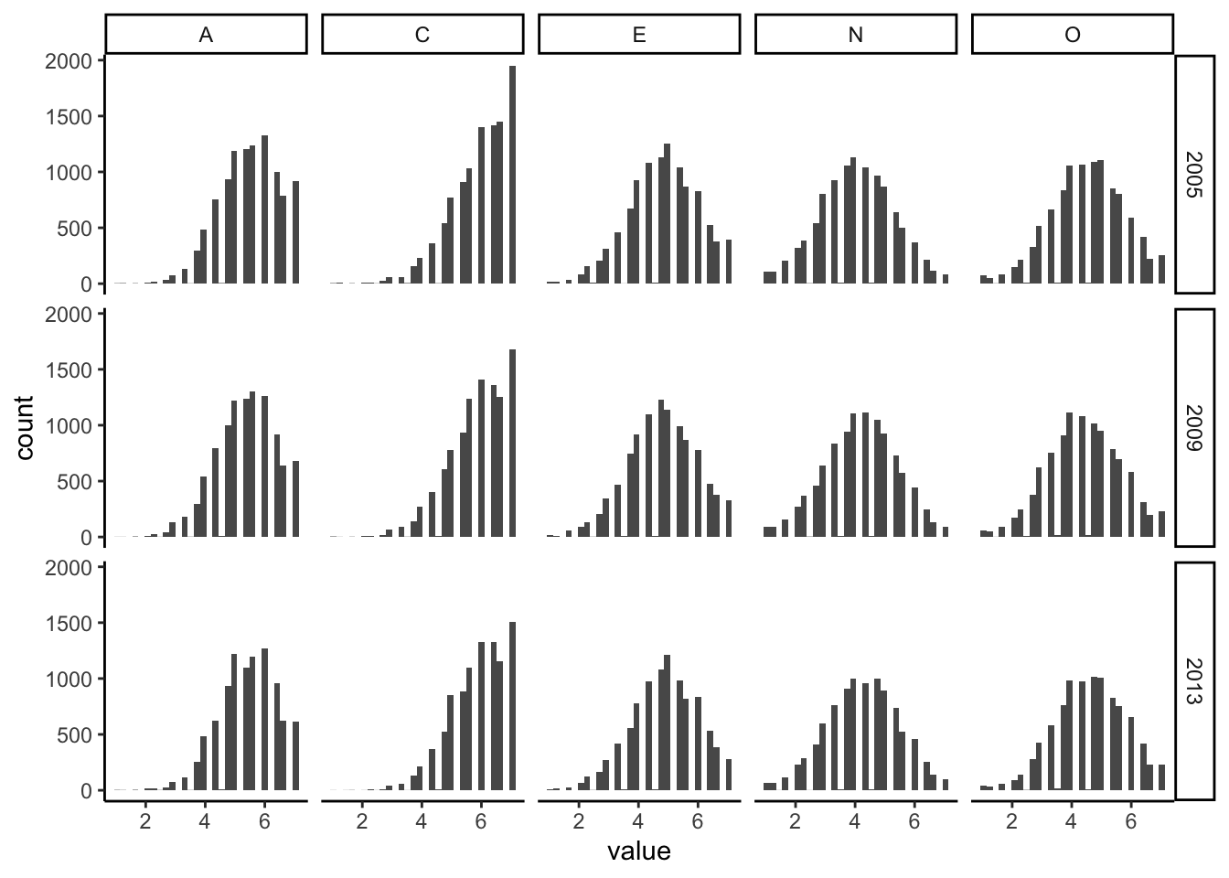
Life Events Descriptives
For count variables, like life events, we need to use something slightly different. We’re typically more interested in counts – in this case, how many people experienced each life event in the 10 years we’re considering?
To do this, we’ll use a little bit of dplyr rather than the base R function table() that is often used for count data. Instead, we’ll use a combination of group_by() and n() to get the counts by group. In the end, we’re left with a nice little table of counts.
events_long %>%
  group_by(item, le_value) %>%
  summarize(N = n()) %>%
  ungroup() %>%
  spread(le_value, N)
# A tibble: 10 × 3
item `0` `1`
<chr> <int> <int>
1 ChldBrth 1600 735
2 ChldMvOut 1555 830
3 DadDied 953 213
4 Divorce 414 122
5 Married 1646 331
6 MomDied 929 219
7 MoveIn 1403 419
8 NewPart 1207 420
9 PartDied 402 76
10 SepPart 1172 415Life Event Plots
events_long %>%
  mutate(le_value = mapvalues(le_value, 0:1, c("No Event", "Event"))) %>%
  ggplot(aes(x = le_value, fill = le_value)) +
    scale_fill_manual(values = c("cornflowerblue", "gray")) +
    geom_bar(color = "black")  +
    facet_wrap(~item, nrow = 2) +
    theme_classic() +
    theme(legend.position = "bottom")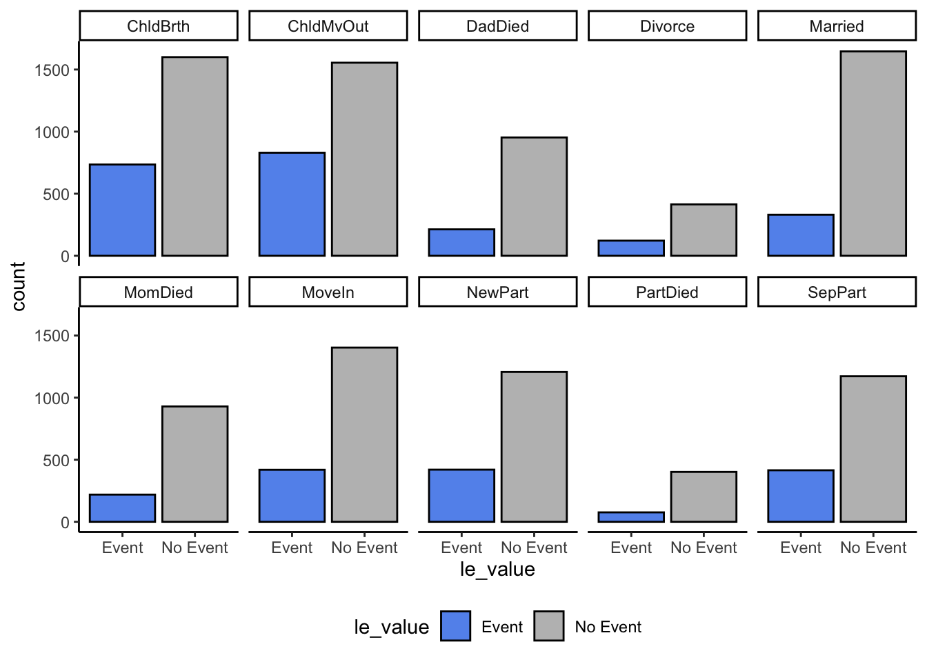
Scale Reliability
When we work with scales, it’s often a good idea to check the internal consistency of your scale. If the scale isn’t performing how it should be, that could critically impact the inferences you make from your data.
To check the internal consistency of our Big 5 scales, we will use the alpha() function from the psych package, which will give us Cronbach’s as well as a number of other indicators of internal consistency.
Here’s the way you may have seen / done this in the past.
alpha.C.2005 <- with(soep, psych::alpha(x = cbind(`Big 5__C_thorough.2005`,
                                  `Big 5__C_lazy.2005`, `Big 5__C_efficient.2005`)))
Some items ( Big 5__C_lazy.2005 ) were negatively correlated with the total scale and
probably should be reversed.
To do this, run the function again with the 'check.keys=TRUE' optionBut again, doing this 15 times would be quite a pain and would open you up to the possibility of a lot of copy and paste errors.
So instead, to do this, I’m going to use a mix of the tidyverse. At first glance, it may seem complex but as you move through other tutorials (particularly the purrr tutorial), it will begin to make much more sense.
# short function to reshape data and run alpha
alpha_fun <- function(df){
  df %>% spread(scrap,value) %>% psych::alpha(.)
}

(alphas <- soep_long %>%
  filter(type == "Big 5") %>% # filter out Big 5
  select(Procedural__SID, item:value) %>% # get rid of extra columns
  group_by(item, year) %>% # group by construct and year
  nest() %>% # nest the data
  mutate(alpha_res = map(data, alpha_fun), # run alpha
         alpha = map(alpha_res, ~.$total[2])) %>% # get the alpha value
  unnest(alpha)) # pull it out of the list column
# A tibble: 15 × 5
# Groups: item, year [15]
item year data alpha_res std.alpha
<chr> <chr> <list> <list> <dbl>
1 C 2005 <tibble [31,117 × 3]> <psych> 0.515
2 C 2009 <tibble [30,728 × 3]> <psych> 0.494
3 C 2013 <tibble [28,496 × 3]> <psych> 0.482
4 E 2005 <tibble [31,188 × 3]> <psych> 0.540
5 E 2009 <tibble [30,770 × 3]> <psych> 0.530
6 E 2013 <tibble [28,532 × 3]> <psych> 0.544
7 A 2005 <tibble [31,184 × 3]> <psych> 0.418
8 A 2009 <tibble [30,796 × 3]> <psych> 0.410
9 A 2013 <tibble [28,529 × 3]> <psych> 0.401
10 O 2005 <tibble [31,091 × 3]> <psych> 0.527
11 O 2009 <tibble [30,722 × 3]> <psych> 0.510
12 O 2013 <tibble [28,451 × 3]> <psych> 0.497
13 N 2005 <tibble [31,162 × 3]> <psych> 0.473
14 N 2009 <tibble [30,802 × 3]> <psych> 0.490
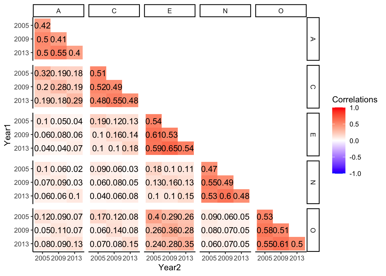
15 N 2013 <tibble [28,536 × 3]> <psych> 0.480Zero-Order Correlations
Finally, we often want to look at the zero-order correlation among study variables to make sure they are performing as we think they should.
To run the correlations, we will need to have our data in wide format, so we’re going to do a little bit of reshaping before we do.
b5_soep_long %>%
  unite(tmp, item, year, sep = "_") %>%
  spread(key = tmp, value = value) %>%
  select(-Procedural__SID) %>%
  cor(., use = "pairwise") %>%
  round(., 2)
DOB Sex A_2005 A_2009 A_2013 C_2005 C_2009 C_2013 E_2005 E_2009
DOB 1.00 0.00 -0.08 -0.07 -0.06 -0.13 -0.12 -0.14 0.10 0.12
Sex 0.00 1.00 0.18 0.17 0.18 0.05 0.07 0.09 0.08 0.08
A_2005 -0.08 0.18 1.00 0.50 0.50 0.32 0.20 0.19 0.10 0.06
A_2009 -0.07 0.17 0.50 1.00 0.55 0.19 0.28 0.18 0.05 0.08
A_2013 -0.06 0.18 0.50 0.55 1.00 0.18 0.19 0.29 0.04 0.06
C_2005 -0.13 0.05 0.32 0.19 0.18 1.00 0.52 0.48 0.19 0.10
C_2009 -0.12 0.07 0.20 0.28 0.19 0.52 1.00 0.55 0.12 0.16
C_2013 -0.14 0.09 0.19 0.18 0.29 0.48 0.55 1.00 0.13 0.14
E_2005 0.10 0.08 0.10 0.05 0.04 0.19 0.12 0.13 1.00 0.61
E_2009 0.12 0.08 0.06 0.08 0.06 0.10 0.16 0.14 0.61 1.00
E_2013 0.10 0.11 0.04 0.04 0.07 0.10 0.10 0.18 0.59 0.65
N_2005 0.06 -0.18 0.10 0.06 0.02 0.09 0.06 0.03 0.18 0.10
N_2009 0.03 -0.22 0.07 0.09 0.03 0.06 0.08 0.05 0.13 0.16
N_2013 0.02 -0.21 0.06 0.06 0.10 0.04 0.06 0.08 0.10 0.10
O_2005 0.11 0.06 0.12 0.09 0.07 0.17 0.12 0.08 0.40 0.29
O_2009 0.10 0.05 0.05 0.11 0.07 0.06 0.14 0.08 0.26 0.36
O_2013 0.05 0.07 0.08 0.09 0.13 0.07 0.08 0.15 0.24 0.28
E_2013 N_2005 N_2009 N_2013 O_2005 O_2009 O_2013
DOB 0.10 0.06 0.03 0.02 0.11 0.10 0.05
Sex 0.11 -0.18 -0.22 -0.21 0.06 0.05 0.07
A_2005 0.04 0.10 0.07 0.06 0.12 0.05 0.08
A_2009 0.04 0.06 0.09 0.06 0.09 0.11 0.09
A_2013 0.07 0.02 0.03 0.10 0.07 0.07 0.13
C_2005 0.10 0.09 0.06 0.04 0.17 0.06 0.07
C_2009 0.10 0.06 0.08 0.06 0.12 0.14 0.08
C_2013 0.18 0.03 0.05 0.08 0.08 0.08 0.15
E_2005 0.59 0.18 0.13 0.10 0.40 0.26 0.24
E_2009 0.65 0.10 0.16 0.10 0.29 0.36 0.28
E_2013 1.00 0.11 0.13 0.15 0.26 0.28 0.35
N_2005 0.11 1.00 0.55 0.53 0.09 0.08 0.06
N_2009 0.13 0.55 1.00 0.60 0.06 0.07 0.07
N_2013 0.15 0.53 0.60 1.00 0.05 0.05 0.05
O_2005 0.26 0.09 0.06 0.05 1.00 0.58 0.55
O_2009 0.28 0.08 0.07 0.05 0.58 1.00 0.61
O_2013 0.35 0.06 0.07 0.05 0.55 0.61 1.00This is a lot of values and a little hard to make sense of, so as a bonus, I’m going to give you a little bit of more complex code that makes this more readable (and publishable ).
r <- b5_soep_long %>%
  unite(tmp, item, year, sep = "_") %>%
  spread(key = tmp, value = value) %>%
  select(-Procedural__SID, -DOB, -Sex) %>%
  cor(., use = "pairwise")

r[upper.tri(r, diag = T)] <- NA
diag(r) <- (alphas %>% arrange(item, year))$std.alpha

r %>% data.frame %>%
  rownames_to_column("V1") %>%
  gather(key = V2, value = r, na.rm = T, -V1) %>%
  separate(V1, c("T1", "Year1"), sep = "_") %>%
  separate(V2, c("T2", "Year2"), sep = "_") %>%
  mutate_at(vars(Year1), ~factor(., levels = c(2013, 2009, 2005))) %>%
  ggplot(aes(x = Year2, y = Year1, fill = r)) +
    geom_raster() +
  scale_fill_gradient2(low = "blue", high = "red", mid = "white",
   midpoint = 0, limit = c(-1,1), space = "Lab",
   name="Correlations") +
  geom_text(aes(label = round(r,2))) +
    facet_grid(T1 ~ T2) +
    theme_classic()