── Attaching core tidyverse packages ──────────────────────── tidyverse 2.0.0 ──
✔ dplyr     1.1.3     ✔ readr     2.1.4
✔ forcats   1.0.0     ✔ stringr   1.5.0
✔ ggplot2   3.4.2     ✔ tibble    3.2.1
✔ lubridate 1.9.3     ✔ tidyr     1.3.0
✔ purrr     1.0.2
── Conflicts ────────────────────────────────────────── tidyverse_conflicts() ──
✖ dplyr::arrange()   masks plyr::arrange()
✖ purrr::compact()   masks plyr::compact()
✖ dplyr::count()     masks plyr::count()
✖ dplyr::desc()      masks plyr::desc()
✖ dplyr::failwith()  masks plyr::failwith()
✖ dplyr::filter()    masks stats::filter()
✖ dplyr::id()        masks plyr::id()
✖ dplyr::lag()       masks stats::lag()
✖ dplyr::mutate()    masks plyr::mutate()
✖ dplyr::rename()    masks plyr::rename()
✖ dplyr::summarise() masks plyr::summarise()
✖ dplyr::summarize() masks plyr::summarize()
ℹ Use the conflicted package (<http://conflicted.r-lib.org/>) to force all conflicts to become errorsIntroduction to ggplot2
Code

What is ggplot2 trying to do?
- Create a grammar of graphics
- Aims to help draw connections across diverse plots
- Create order in the chaos of complicated plots
From Wickham (2010):
A grammar of graphics is a tool that enables us to concisely describe the components of a graphic.
What are the core elements of ggplot2 grammar?
- Mappings: base layer
- Scales: control and modify your mappings
- Geoms: plot elements
- Facets: panel your plot
- Grobs: things that aren’t geoms that we want to layer on like text, arrows, other things
- Themes: style your figure
But first, our data
- These are some Experience Sampling Method data I collected during my time in graduate school
- Specifically, these include data from Beck & Jackson (2022)
- In that paper I built personalized machine learning models of behaviors and experiences from sets of:
- psychological
- situational
- and time variables
Code
Mappings
- The first thing we call with
ggplot2is always theggplot()function, which has two core arguments:-
data: your data object (can also be piped)
-

-
mapping: your aesthetic mappings for the plot, wrapped inaes()
- How many aesthetic mappings are there?
xy-
col/color fillshapesizelinetype-
xmin/xmax -
ymin/ymax alpha
- There are lots of geom-specific ones, too
- Use ?geom_whatever() to get more info on a specific geom
Scales
- Every mapping is a scale
- Scales can be lots of different things
- In ggplot2 language, some core ones are:
continuousdiscretemanualordinalbinneddatebrewer
- All of these have specific arguments based on the type of scale
continuous
- Let’s try the
continuousscale with ourymapping - We’ll use the following three arguments
-
limits: vector length 2 -
breaks: vector of any length -
labels: numeric or character vector
-
Geoms
- We’ll loop back to scales after talking about some geoms
- It’s not possible to go through all the possible geoms (that’s what the rest of the class is for!)
- We’ll focus on some basic ones for now
geom_point()geom_jitter()geom_smooth()-
geom_hline()/geom_vline() geom_bar()geom_boxplot()geom_density()geom_histogram()
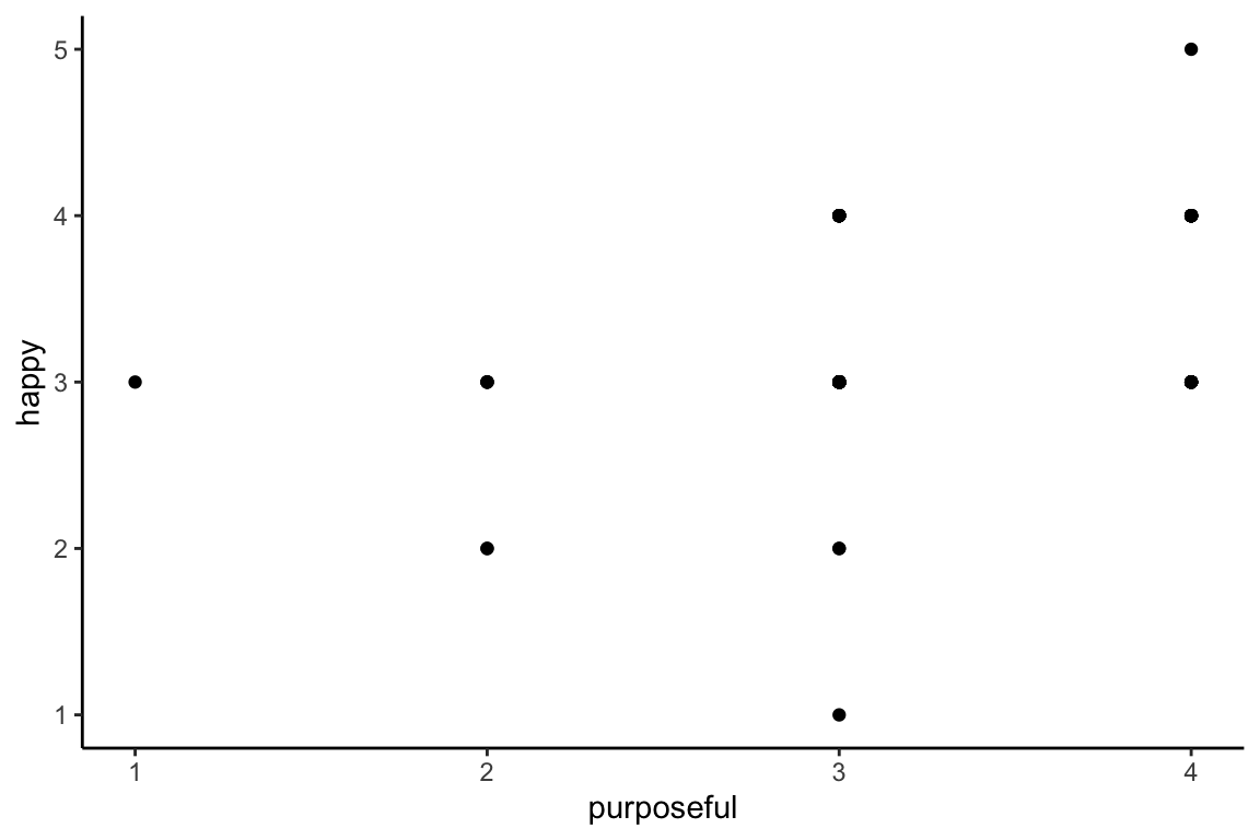
##geom_point()
Your basic scatterplot!
Code
Let’s add color:
Code
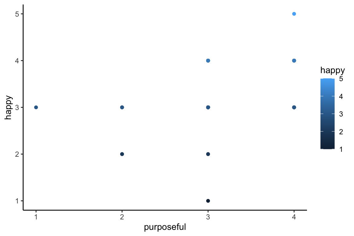
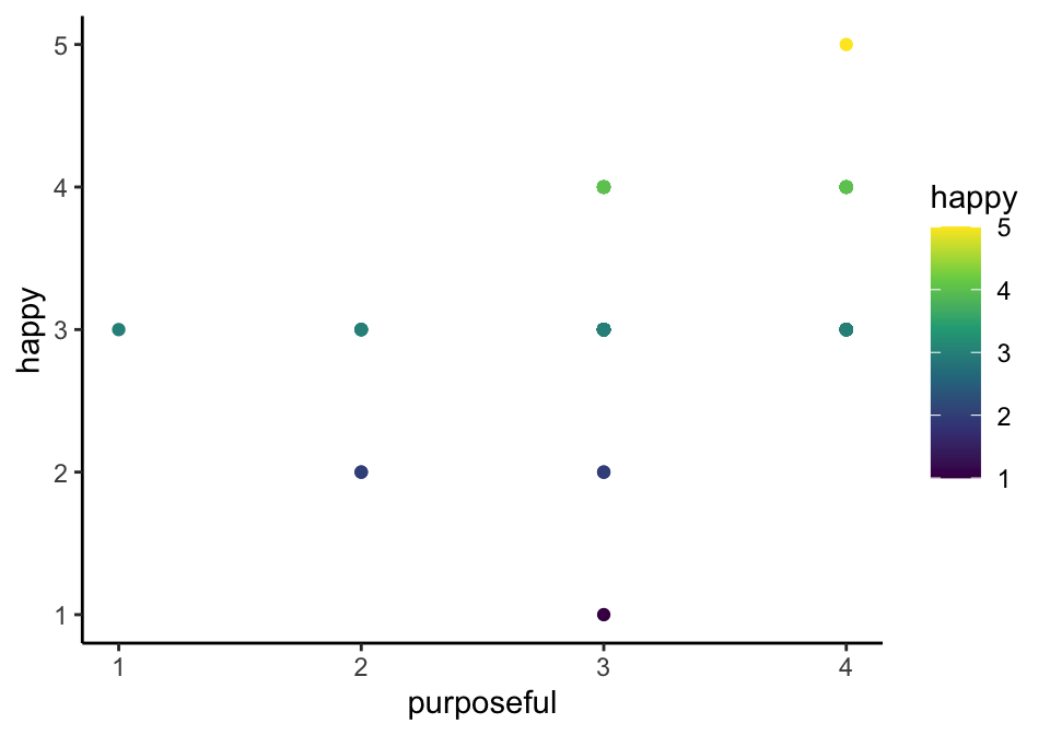
And change the scale using built-in types.
Code
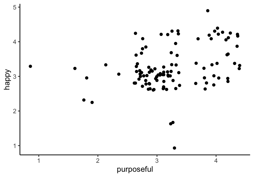
geom_jitter()
- Sometimes we have data that have lots of repeating values, especially with ordinal response scales where the variables aren’t composited / latent
- jitter adds random noise to the point to allow you to see more of the points
Code
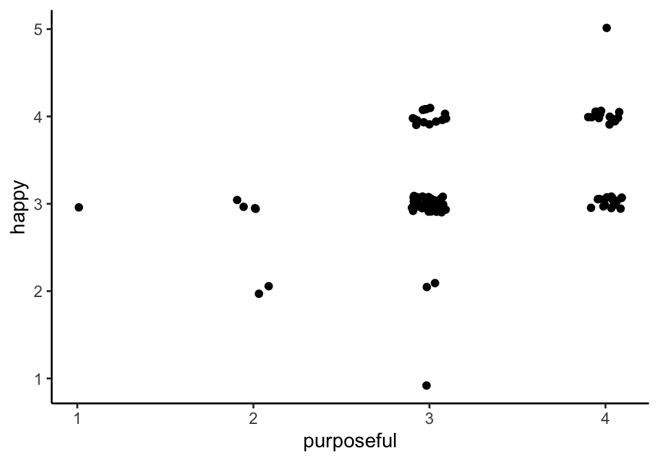
This may be too much jitter
- Sometimes we have data that have lots of repeating values, especially with ordinal response scales where the variables aren’t composited / latent
- jitter adds random noise to the point to allow you to see more of the points
Code
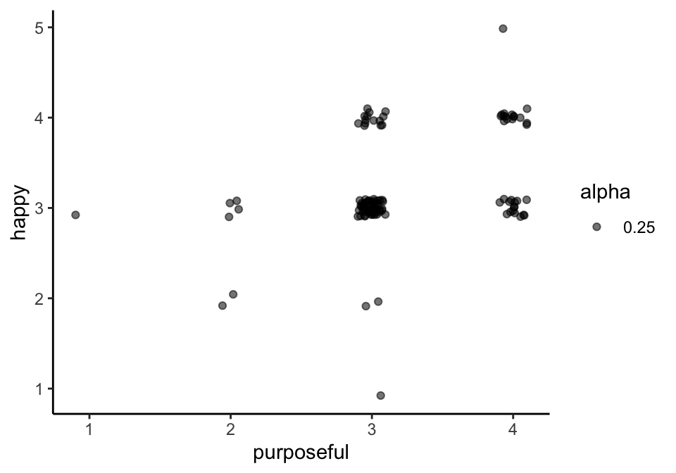
alpha
Alpha can help us understand how many points are stacked when using jitter (or other overlapping data)
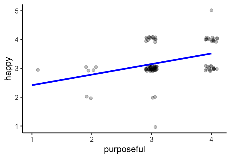
geom_smooth()
-
geom_smooth()allows you to apply statistical functions to your data - There are other ways to do this that we won’t cover today
- Core arguments are:
-
method: “loess”, “lm”, “glm”, “gam” -
formula: e.g.,y ~ xory ~ poly(x, 2) -
se: display standard error of estimate (T/F) -
aes()wrapped aesthetics or directly mapped aesthetics
-
Remember: it’s a LAYERED grammar of graphics, so let’s layer!
se = F
method = "lm"
method = "loess"
Code
Warning in simpleLoess(y, x, w, span, degree = degree, parametric = parametric,
: pseudoinverse used at 4.015
Warning in simpleLoess(y, x, w, span, degree = degree, parametric = parametric,
: neighborhood radius 1.015Warning in simpleLoess(y, x, w, span, degree = degree, parametric = parametric,
: reciprocal condition number 0Warning in simpleLoess(y, x, w, span, degree = degree, parametric = parametric,
: There are other near singularities as well. 1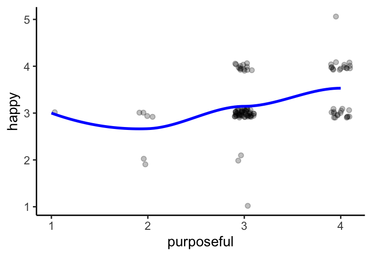
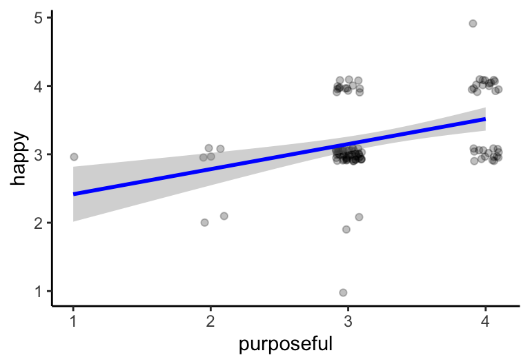
se=T
And we can add standard error ribbons
method = "lm"
method = "loess"
Code
Warning in simpleLoess(y, x, w, span, degree = degree, parametric = parametric,
: pseudoinverse used at 4.015
Warning in simpleLoess(y, x, w, span, degree = degree, parametric = parametric,
: neighborhood radius 1.015Warning in simpleLoess(y, x, w, span, degree = degree, parametric = parametric,
: reciprocal condition number 0Warning in simpleLoess(y, x, w, span, degree = degree, parametric = parametric,
: There are other near singularities as well. 1Warning in predLoess(object$y, object$x, newx = if (is.null(newdata)) object$x
else if (is.data.frame(newdata))
as.matrix(model.frame(delete.response(terms(object)), : pseudoinverse used at
4.015Warning in predLoess(object$y, object$x, newx = if (is.null(newdata)) object$x
else if (is.data.frame(newdata))
as.matrix(model.frame(delete.response(terms(object)), : neighborhood radius
1.015Warning in predLoess(object$y, object$x, newx = if (is.null(newdata)) object$x
else if (is.data.frame(newdata))
as.matrix(model.frame(delete.response(terms(object)), : reciprocal condition
number 0Warning in predLoess(object$y, object$x, newx = if (is.null(newdata)) object$x
else if (is.data.frame(newdata))
as.matrix(model.frame(delete.response(terms(object)), : There are other near
singularities as well. 1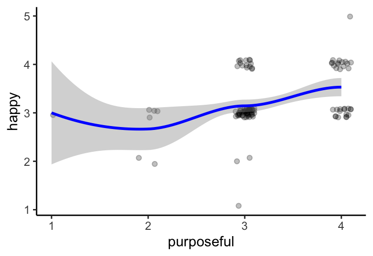
geom_hline()/geom_vline()
- Sometimes, we will want to place lines at various intercepts
- We’ll get into specific use cases as the course progresses
-
geom_hline(): horizontal lines haveyinterceptmappings -
geom_vline(): vertical lines havexinterceptmappings
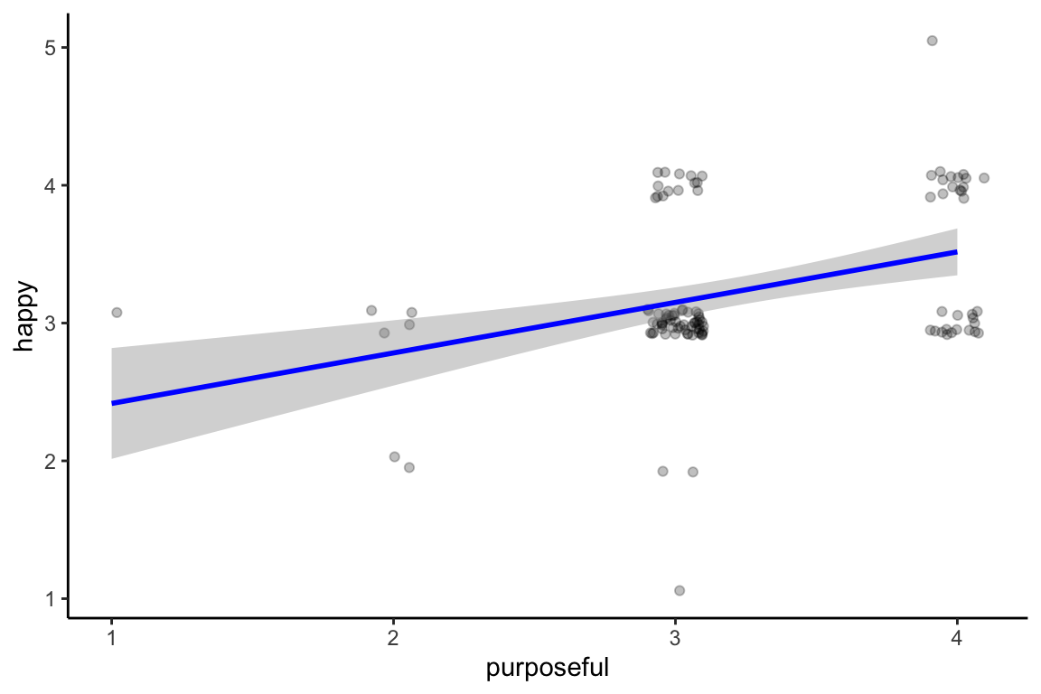
geom_hline()
Horizontal lines have yintercept mappings
Code
ipcs_data %>%
  filter(SID == "216") %>%
  ggplot(mapping = aes(x = purposeful, y = happy)) +
    geom_jitter(width = .1, height = .1, alpha = .25) +
    geom_hline(
      aes(yintercept = mean(happy, na.rm = T))
      , linetype = "dashed"
      ) +
    geom_smooth(method = "lm", formula = y ~ x, se = F, color = "blue") +
    theme_classic() # I just hate grey backgrounds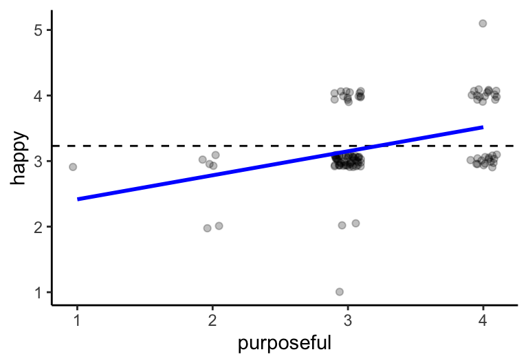
geom_vline()
Vertical lines have xintercept mappings
Code
ipcs_data %>%
  filter(SID == "216") %>%
  ggplot(mapping = aes(x = purposeful, y = happy)) +
    geom_jitter(width = .1, height = .1, alpha = .25) +
    geom_vline(
      aes(xintercept = mean(purposeful, na.rm = T))
      , linetype = "dashed"
      ) +
    geom_smooth(method = "lm", formula = y ~ x, se = F, color = "blue") +
    theme_classic() # I just hate grey backgrounds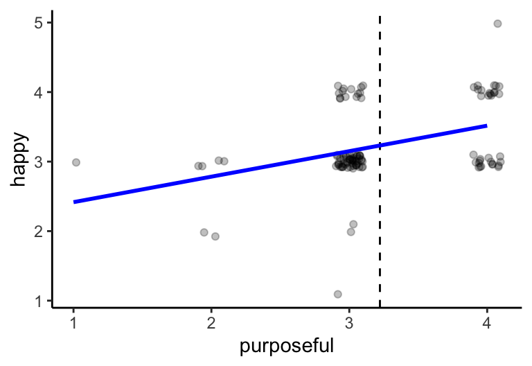
geom_bar()
- Bar graphs can be useful for showing relative differences
- My hot take is that they are rarely that useful
- (This is mostly because of how we perceive errorbars and differences, which we’ll talk more about in a few weeks!)
- But let’s look at using them for frequency and means / se’s
Frequency
How often did our participant have an argument, interact with others, study, and feel tired?
Code
ipcs_data %>%
  filter(SID == "216") %>%
  select(SID, Full_Date, argument, interacted, study, tired) %>%
  pivot_longer(
    cols = argument:tired
    , names_to = "item"
    , values_to = "value"
    , values_drop_na = T
  ) %>%
  group_by(item) %>%
  summarize(value = sum(value == 1)) %>%
  ggplot(aes(x = item, fill = item, y = value)) +
    geom_col(color = "black") +
    theme_classic()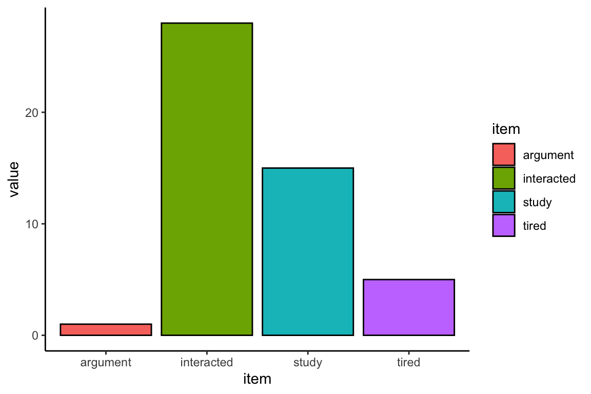
Mean differences
Were there mean-level in our continuous variables?
Code
ipcs_data %>%
  filter(SID %in% c("216")) %>%
  select(SID, Full_Date, happy, purposeful, afraid, attentive) %>%
  pivot_longer(
    cols = c(-SID, -Full_Date)
    , names_to = "item"
    , values_to = "value"
    , values_drop_na = T
  ) %>%
  group_by(item) %>%
  summarize(
    mean = mean(value)
    , ci = 1.96*(sd(value)/sqrt(n()))
    ) %>%
  ggplot(aes(x = item, fill = item, y = mean)) +
    geom_col(color = "black") +
    geom_errorbar(
      aes(ymin = mean - ci, ymax = mean + ci)
      , position = position_dodge(width = .1)
      , width = .1
      , stat = "identity"
    ) +
    theme_classic()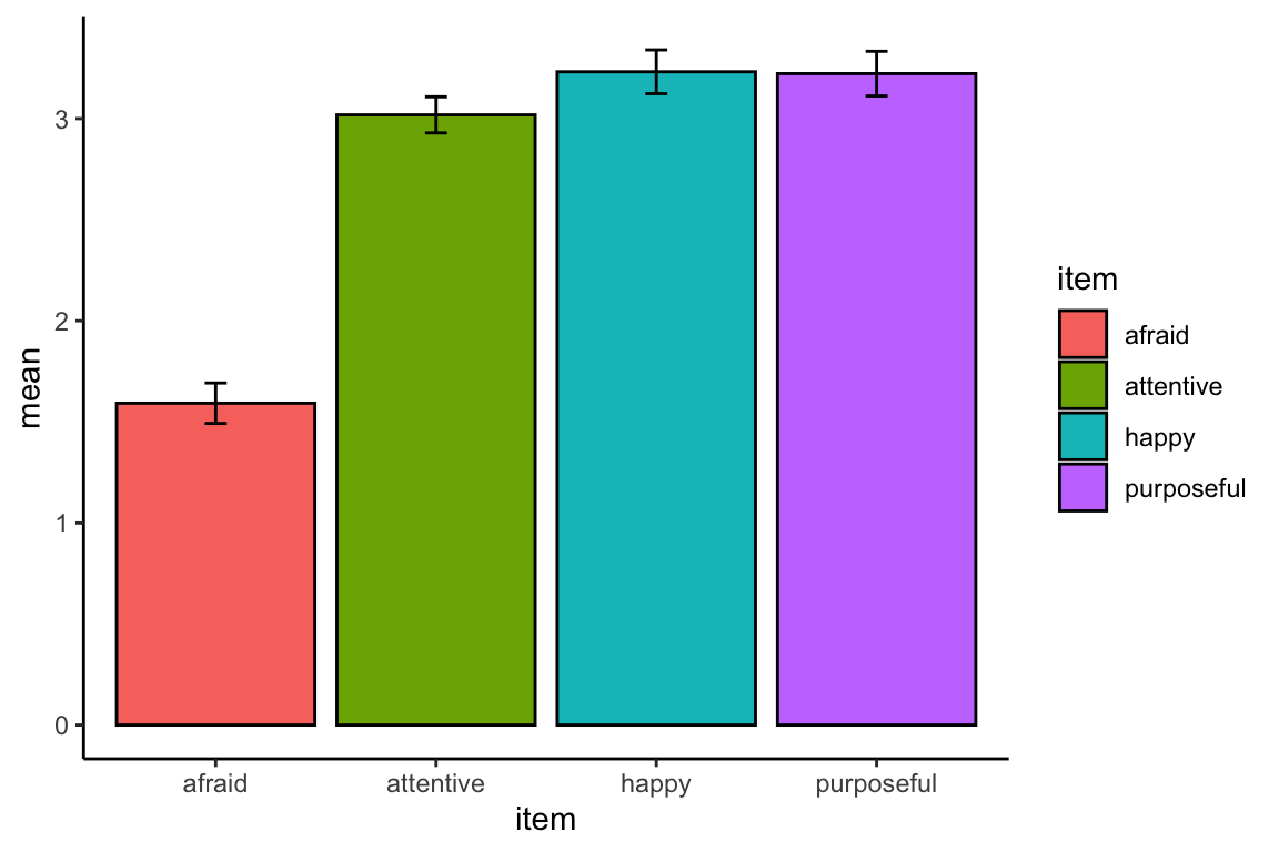
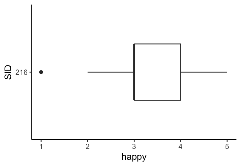
geom_boxplot()
- Sometimes called box and whisker plots
- A method for summarizing a distribution of data without showing raw data
- Box instead shows 25th, 50th, and 75th percentile (quartiles)
- Whiskers show 1.5 * interquartile range (75%tile-25%tile)
- More fun when we want to compare distributions across variables (IMO)
One boxplot
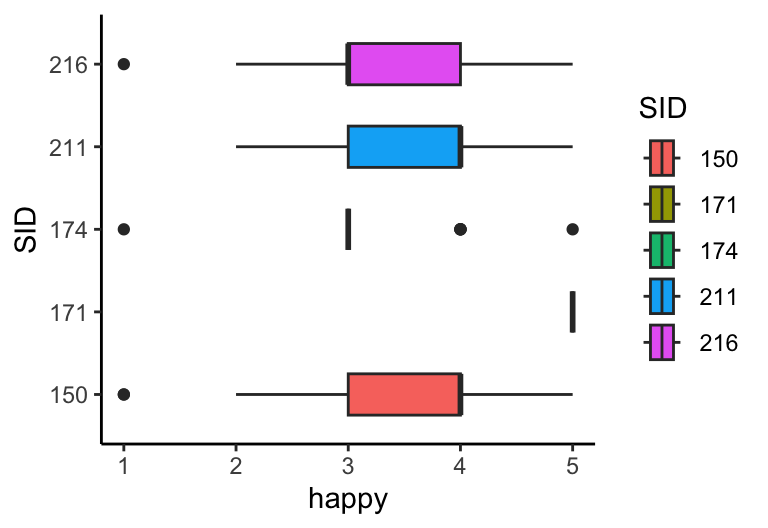
Multiple boxplots
Multiple Participants
- Later, we’ll also talk about how to order the boxplots (and other axes) by means, medians, etc.
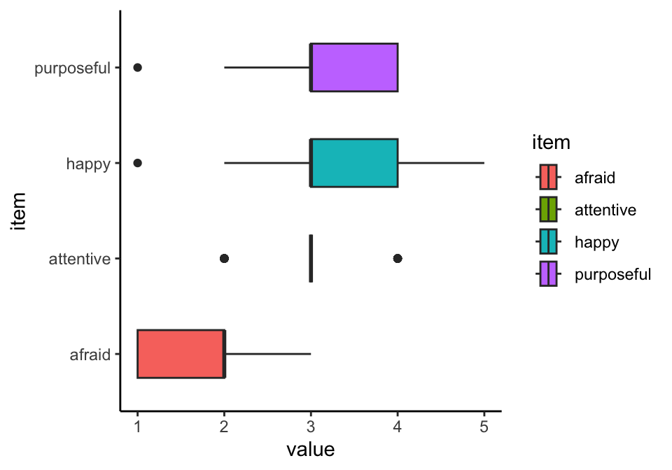
Multiple Variables
Advanced!
Code
ipcs_data %>%
  filter(SID == "216") %>%
  ggplot(mapping = aes(x = purposeful, y = happy)) +
    scale_x_continuous(limits = c(1,7), breaks = seq(1,5,2)) +
    scale_y_continuous(limits = c(1,7), breaks = seq(1,5,2)) +
    geom_jitter(width = .1, height = .1, alpha = .25) +
    geom_boxplot(aes(
      x = 6
      , y = happy
      )) +
    geom_boxplot(aes(
      y = 6
      , x = purposeful
      )) +
    geom_smooth(
      method = "lm"
      , formula = y ~ x
      , se = F
      , color = "blue"
      ) +
    theme_classic() # I just hate grey backgrounds
Warning: Removed 1 rows containing missing values (`geom_point()`).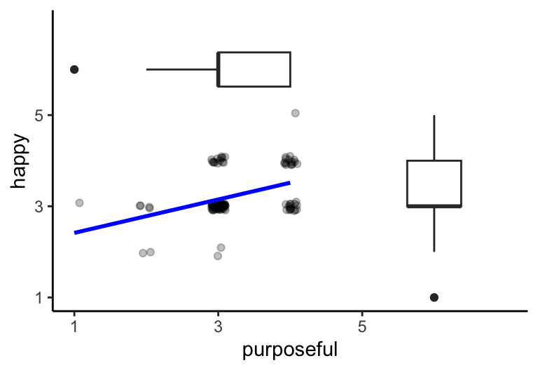
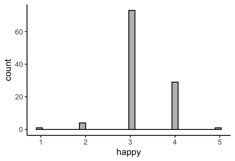
geom_histogram() & geom_density()
- Useful for showing raw / smoothed distributions of data
Histogram
Density Distribution
Code
Warning: The dot-dot notation (`..density..`) was deprecated in ggplot2 3.4.0.
ℹ Please use `after_stat(density)` instead.
`stat_bin()` using `bins = 30`. Pick better value with `binwidth`.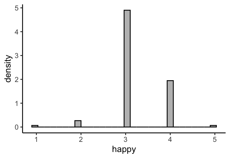
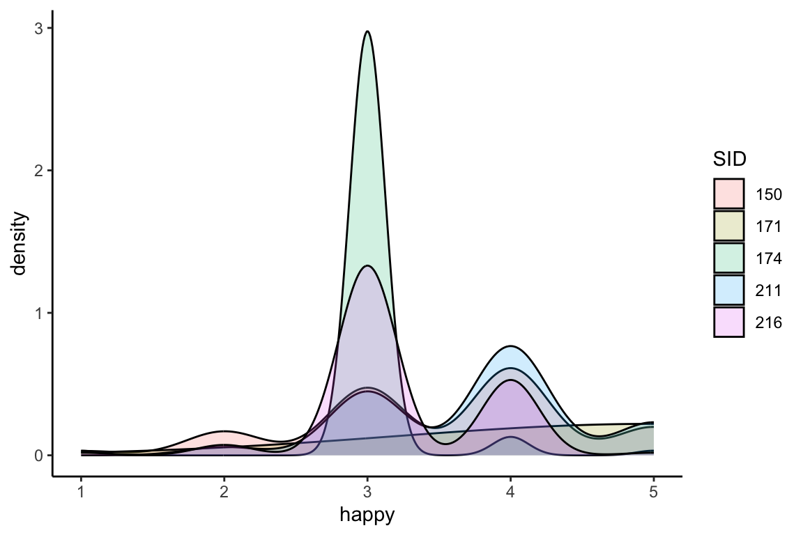
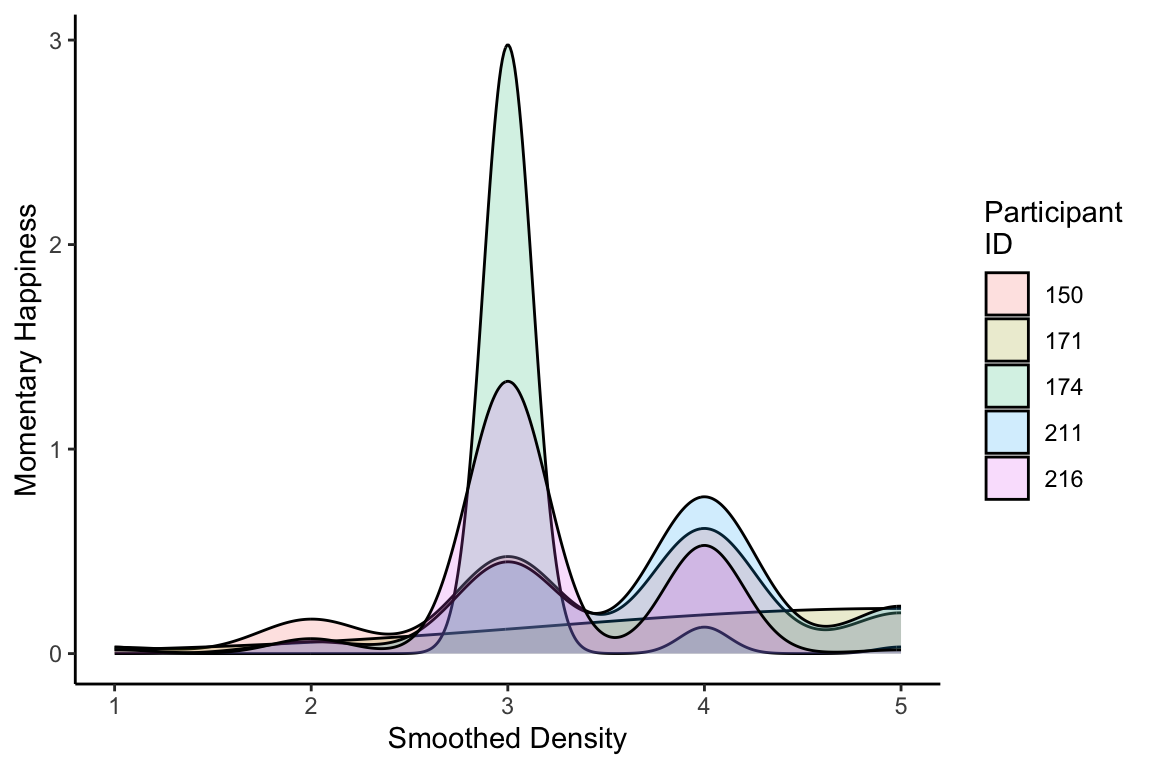
Multiple histograms / density distributions
- We can compare multiple participants
Plot Appearance Beyond Mappings
- So far, we have only changed appearance via the
scale_()functions - But that doesn’t change things like axis, text, title, and more
- Nor does it help when we want to split the plot into multiple panels
- Let’s do those next!
Facets
- Often, we have lots of other reasons we need to reproduce the same plot multiple times
- multiple variables
- multiple people
- multiple conditions
- etc.
- There are more ways to do this than we’ll cover today, like piecing plots together and more
- The core of directly faceting within ggplot is that you have to facet according to variables in your data set
- This is part of why we covered moving your data to long
- Say that you want to facet by variable, for example, but your data is in wide form
- Facets couldn’t handle that
Code
In ggplot2, there are two core faceting functions * facet_grid() + snaps figures in a grid; no wrapping + especially useful for 1-2 faceting variables * facet_wrap() + treats each facet a separate + wraps according to nrow and ncol arguments
facet_grid()
Core arguments:
-
rows,cols: list of variables or formula, e.g.,x ~ y -
scales: same x or y scale on all facets? -
space: same space for unequal length x or y facets? -
switch: move labels from left to right or top to bottom? -
drop: drop unused factor levels

facet_wrap()
Core arguments:
-
facets: barequoted or one-sided formula, e.g.,~ x + y -
nrow/ncol: number of rows and columns -
scales: same x or y scale on all facets? -
switch: move labels from left to right or top to bottom? -
drop: drop unused factor levels -
dir: horizontal or vertical -
strip.position: where to put the labels
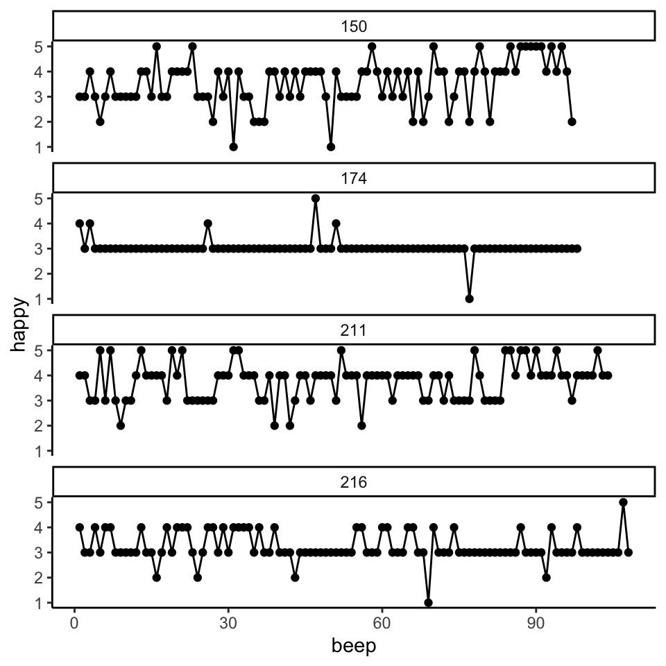
Code
ipcs_data %>%
  filter(SID == "216") %>%
  select(SID, beep, afraid:content) %>%
  pivot_longer(
    cols = afraid:content
    , names_to = "item"
    , values_to = "value"
) %>%
ggplot(aes(x = beep, y = value, group = item)) +
geom_point() +
geom_line() +
facet_wrap(
~item
, ncol = 1
, strip.position = "right"
) +
theme_classic()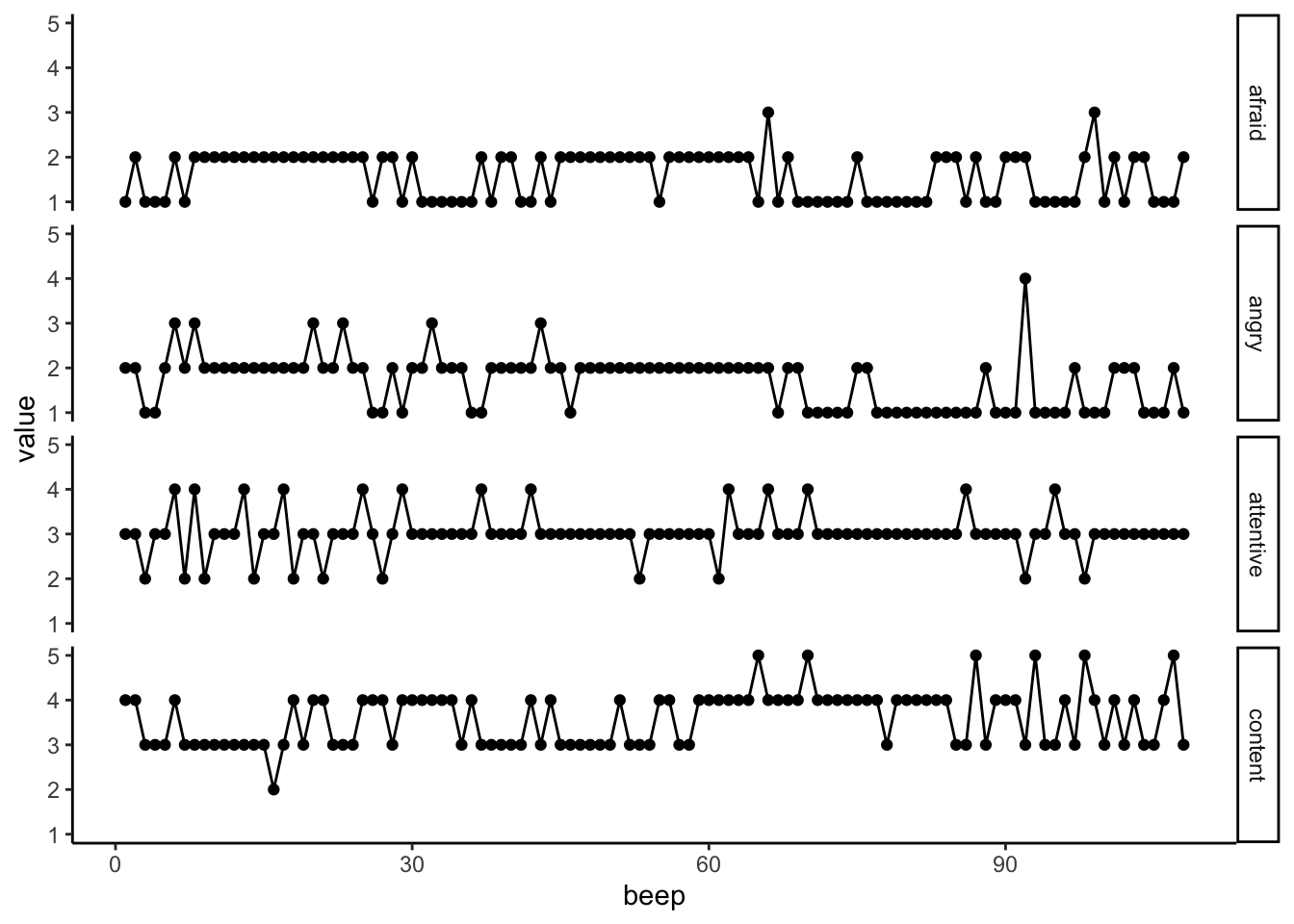
Change scale and space
Code
ipcs_data %>%
  filter(SID == "216") %>%
  select(SID, beep, afraid:content) %>%
  pivot_longer(
    cols = afraid:content
    , names_to = "item"
    , values_to = "value"
  ) %>%
  ggplot(aes(x = beep, y = value, group = item)) +
    geom_point() +
    geom_line() +
    facet_grid(
      item ~ .
      , scales = "free_y"
      , space = "free_y"
      ) +
    theme_classic()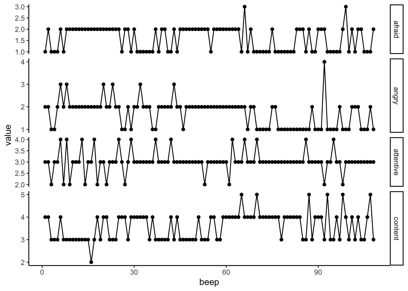
Labels & Titles
- APA style says titles are bad
- Common sense says titles help understanding
- Ask for forgiveness, not permission
Remember this?
Code
We can add labels and a title
Code
ipcs_data %>%
  filter(SID == "216") %>%
  ggplot(mapping = aes(x = purposeful, y = happy)) +
    geom_jitter(width = .1, height = .1, alpha = .25) +
    geom_smooth(
      method = "lm"
      , formula = y ~ x
      , se = T
      , color = "blue"
    ) +
    labs(
      x = "Momentary Purpose (1-5)"
      , y = "Momentary Happiness (1-5)"
      , title = "Zero-Order Associations
                  Between Momentary Happiness and Purpose"
    ) +
    theme_classic() # I just hate grey backgrounds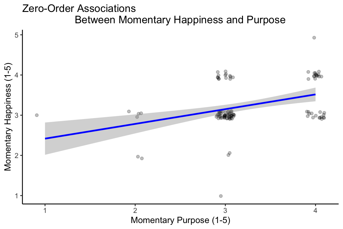
Labels also apply to other mappings like color
Code
You can also use labels to remove axis labels
Code
ipcs_data %>%
  filter(SID %in% c("216")) %>%
  select(SID, Full_Date, happy, purposeful, afraid, attentive) %>%
  pivot_longer(
    cols = c(-SID, -Full_Date)
    , names_to = "item"
    , values_to = "value"
  ) %>%
  ggplot(aes(
    y = item
    , x = value
    , fill = item
    )) +
    geom_boxplot(width = .5) +
    labs(
      x = "Momentart Rating (1-5)"
      , y = NULL
      , fill = "Item"
    ) +
    theme_classic()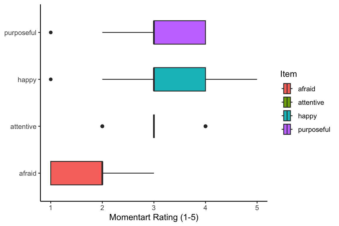
Themes
Basic, Built-in Themes
- There are lots of themes you can use in ggplot that are pre-built into the package
- Try tying
theme_into your R console, and look at the functions that pop up - Some stand-out ones are:
-
theme_classic()(what we’ve been using) theme_bw()-
theme_minimal()(but is there a theme_maximal?) theme_void
-
Advanced Themes
- Custom themes are one of the best ways to “hack” your ggplots
- You will not remember all of them
- You will have to google them all time
- Here’s the site: https://ggplot2.tidyverse.org/reference/theme.html
- Rather than give details on a bunch of these, I’m going to demonstrate theme modifications I often use
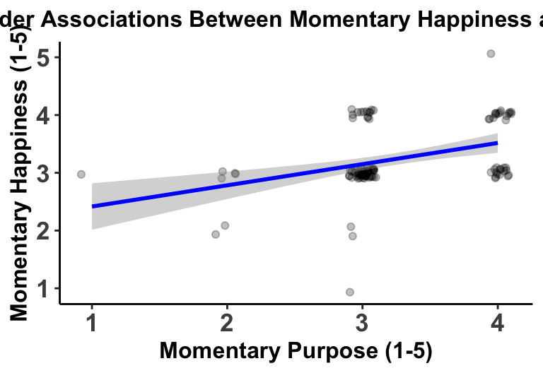
Smoothed Regression Line
Code
ipcs_data %>%
  filter(SID == "216") %>%
  ggplot(mapping = aes(x = purposeful, y = happy)) +
    geom_jitter(width = .1, height = .1, alpha = .25) +
    geom_smooth(
      method = "lm"
      , formula = y ~ x
      , se = T
      , color = "blue"
    ) +
    labs(
      x = "Momentary Purpose (1-5)"
      , y = "Momentary Happiness (1-5)"
      , title = "Zero-Order Associations Between Momentary Happiness and Purpose"
    ) +
    theme_classic() +
    theme(
      plot.title = element_text(
        face = "bold"
        , size = rel(1.1)
        , hjust = .5
        )
      , axis.title = element_text(
        face = "bold"
        , size = rel(1.1)
        )
      , axis.text = element_text(
        face = "bold"
        , size = rel(1.2)
        )
    )
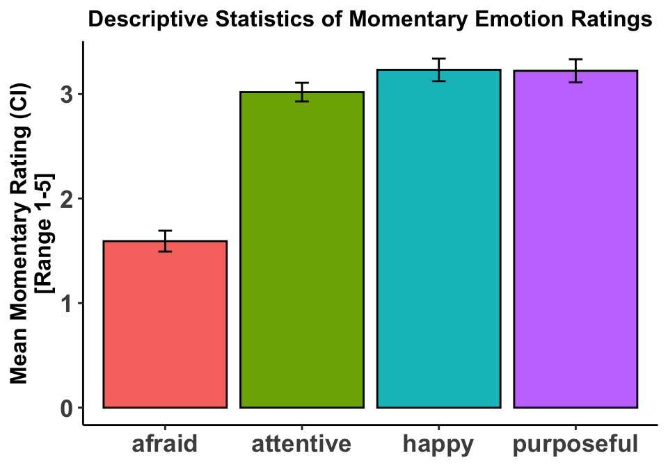
Bar Chart
Code
ipcs_data %>%
  filter(SID %in% c("216")) %>%
  select(SID, Full_Date, happy, purposeful, afraid, attentive) %>%
  pivot_longer(
    cols = c(-SID, -Full_Date)
    , names_to = "item"
    , values_to = "value"
    , values_drop_na = T
  ) %>%
  group_by(item) %>%
  summarize(
    mean = mean(value)
    , ci = 1.96*(sd(value)/sqrt(n()))
    ) %>%
  ggplot(aes(x = item, fill = item, y = mean)) +
    geom_col(color = "black") +
    geom_errorbar(
      aes(ymin = mean - ci, ymax = mean + ci)
      , position = position_dodge(width = .1)
      , width = .1
      , stat = "identity"
    ) +
    labs(
      x = NULL
      , y = "Mean Momentary Rating (CI)\n[Range 1-5]"
      , title = "Descriptive Statistics of Momentary Emotion Ratings"
    ) +
    theme_classic() +
    theme(
      legend.position = "none"
      , plot.title = element_text(face = "bold", size = rel(1.1), hjust = .5)
      , axis.title = element_text(face = "bold", size = rel(1.1))
      , axis.text = element_text(face = "bold", size = rel(1.2))
  )
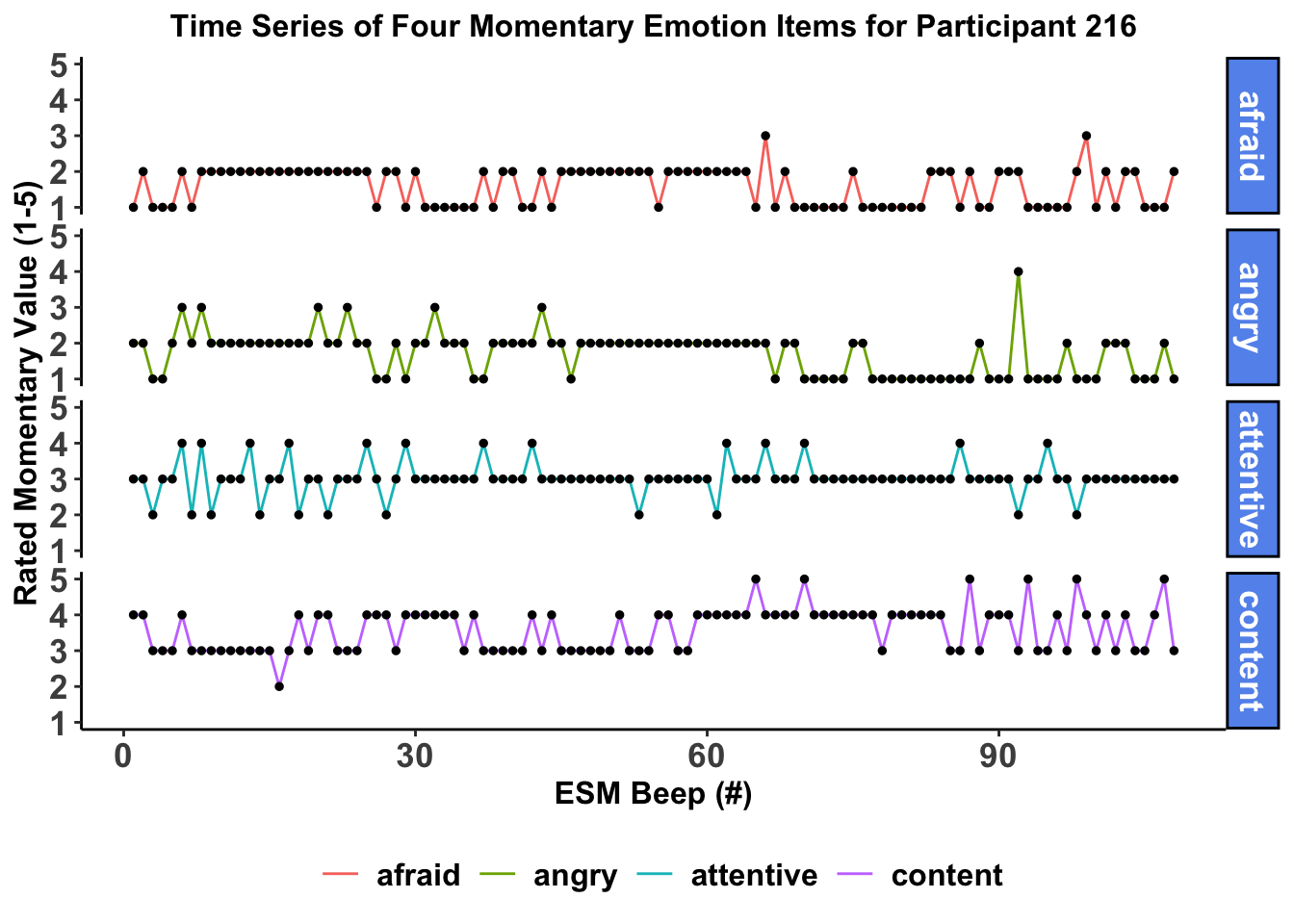
Time Series
Code
ipcs_data %>%
  filter(SID == "216") %>%
  select(SID, beep, afraid:content) %>%
  pivot_longer(
    cols = afraid:content
    , names_to = "item"
    , values_to = "value"
  ) %>%
  ggplot(aes(x = beep, y = value, group = item)) +
    geom_line(aes(color = item)) +
    geom_point(size = 1) +
    facet_grid(item~.) +
    labs(
      x = "ESM Beep (#)"
      , y = "Rated Momentary Value (1-5)"
      , title = "Time Series of Four Momentary Emotion Items for Participant 216"
      , color = NULL
      ) +
    theme_classic() +
    theme(
      legend.position = "bottom"
      , legend.text = element_text(face = "bold", size = rel(1.1))
      , plot.title = element_text(face = "bold", size = rel(1.1), hjust = .5)
      , axis.title = element_text(face = "bold", size = rel(1.1))
      , axis.text = element_text(face = "bold", size = rel(1.2))
      , strip.background = element_rect(color = "black", fill = "cornflowerblue")
      , strip.text = element_text(face = "bold", size = rel(1.2), color = "white")
    )